Supervised forecasting with forecast_pairs#
Predicting a future move from features known now is a supervised-learning problem,
and its classic trap is leakage: pairing a feature at time t with a target that
secretly peeks past t. forecast_pairs builds the training set without that risk.
Its trick is to lag the features rather than lead the target: it never shifts a
value backward in time, so nothing here sees the future. The target must itself be
causal (a trailing quantity, known as-of its own bar).
import numpy as np
import matplotlib.pyplot as plt
from screamer import (RollingSum, RollingLinearRegression,
                      BacktestPriceTarget, backtest_report, RollingSharpe)
from screamer.supervised import forecast_pairs

# A synthetic market with a genuine, learnable edge. `sig` is an observable,
# persistent signal (an AR(1) process, e.g. a normalized spread). The next bar's
# return reverts against it: when the signal is high, price tends to drift down.
rng = np.random.default_rng(7)
n = 8000
phi = 0.95
sig = np.zeros(n)
for t in range(1, n):
    sig[t] = phi * sig[t - 1] + rng.standard_normal()

k = 0.6
eps = rng.standard_normal(n) * 3.0
ret = np.empty(n); ret[0] = 0.0
ret[1:] = -k * sig[:-1] + eps[1:]          # ret[t] is driven by sig[t-1] (known at t-1)
price = 100.0 + np.cumsum(ret)             # a positive price to mark positions against
print(f"{n} bars; the signal explains a real, fadeable part of the next return")
8000 bars; the signal explains a real, fadeable part of the next return
Features and a causal target#
The features are whatever a model reads at time t: here the signal itself plus a
noisier proxy of it, so the fit has to learn which one matters. The target is
the thing we want to predict, the next h-bar return. We express it as a trailing
RollingSum of returns, which is causal at every bar; forecast_pairs shifts it
into the future for us. Writing a forward sum by hand is exactly where the
off-by-one leakage creeps in, which is the step forecast_pairs takes over.
feat2 = sig + rng.standard_normal(n) * 2.0        # a noisy proxy of the signal
X = np.column_stack([sig, feat2])                 # (n, 2) feature matrix

h = 5
y = np.asarray(RollingSum(h)(ret))                # trailing h-bar return, causal
print("features:", X.shape, " target:", y.shape)
features: (8000, 2) target: (8000,)
The leak-safe pairing#
forecast_pairs(X, y, count=h) pairs the features from h bars ago with the target
now: row t holds (X[t-h], y[t]), so a model that reads today's features learns to
predict h bars ahead. It returns (X_shifted, y, as_of), where as_of is each
row's completion time, the bar at which its target is realized. dropna=True
returns a clean training set: it drops the warmup rows (no feature exists h bars
before the start) and any row whose features or target are NaN.
Xs, ys, as_of = forecast_pairs(X, y, count=h, dropna=True)
print(f"{len(Xs)} training rows, {Xs.shape[1]} features")
print(f"as_of spans bars {as_of.min()}..{as_of.max()} (the warmup head is dropped)")
7995 training rows, 2 features
as_of spans bars 5..7999 (the warmup head is dropped)
Train / test split with an embargo#
Because every example carries its as_of completion time, a chronological split is
straightforward: train on early rows, test on late ones. The one subtlety is the
seam: two examples straddling the boundary share overlapping target windows (each
target sums h bars), so we drop h rows at the split, an embargo, so no test
information touches training. Then a plain least-squares fit regresses the target on
the features. A single hold-out gives a first read; production studies use
walk-forward validation across many windows to avoid overfitting to one split.
cut = as_of[int(0.6 * len(as_of))]
train = as_of < cut - h                           # embargo: drop h rows at the seam
test  = as_of >= cut

def fit(Xt, yt):
    A = np.column_stack([np.ones(len(Xt)), Xt])
    coef, *_ = np.linalg.lstsq(A, yt, rcond=None)
    return coef

def predict(coef, Xm):
    return np.column_stack([np.ones(len(Xm)), Xm]) @ coef

coef = fit(Xs[train], ys[train])
pred_test = predict(coef, Xs[test])

corr = np.corrcoef(pred_test, ys[test])[0, 1]
r2 = 1 - np.sum((ys[test] - pred_test) ** 2) / np.sum((ys[test] - ys[test].mean()) ** 2)
print(f"coefficients [intercept, sig, feat2] = {np.round(coef, 3)}")
print(f"  the sig weight is negative: the model learned to FADE the signal")
print(f"out-of-sample corr(pred, realized) = {corr:+.3f}   R2 = {r2:+.3f}")
coefficients [intercept, sig, feat2] = [ 0.318 -2.751  0.048]
  the sig weight is negative: the model learned to FADE the signal
out-of-sample corr(pred, realized) = +0.774   R2 = +0.599
Prediction quality#
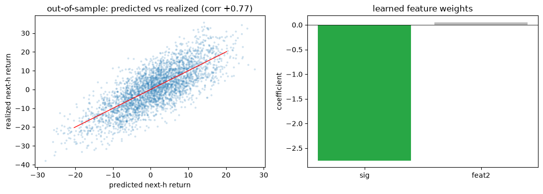
On the untouched test split the prediction lines up with the realized next-h-bar
return, and the model has correctly put almost all of its weight on the true signal
rather than its noisy proxy. The edge is baked into the synthetic data, so the
out-of-sample R2 here is far higher than any real market (where it is often a
fraction of a percent).
fig, ax = plt.subplots(1, 2, figsize=(11, 4))
ax[0].scatter(pred_test, ys[test], s=4, alpha=0.15)
lo, hi = np.percentile(pred_test, [1, 99])
ax[0].plot([lo, hi], [lo, hi], "r", lw=1)
ax[0].set(title=f"out-of-sample: predicted vs realized (corr {corr:+.2f})",
          xlabel="predicted next-h return", ylabel="realized next-h return")
ax[1].bar(["sig", "feat2"], coef[1:], color=["#28a745", "#bbbbbb"])
ax[1].axhline(0, color="k", lw=0.6)
ax[1].set(title="learned feature weights", ylabel="coefficient")
fig.tight_layout()
From a prediction to a backtest#
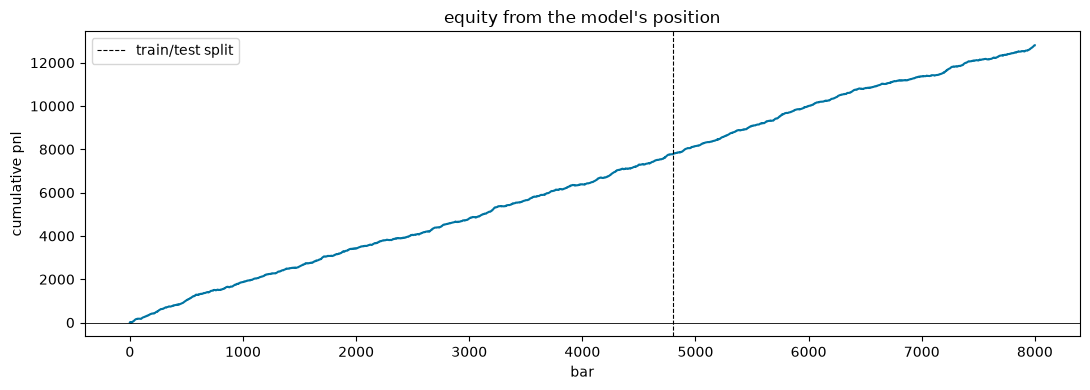
The prediction is a per-bar view of the next move, so it drops straight into the
backtest family. Feed the current features to the fitted model at every bar, take a
position from the sign of the prediction (fade when it expects a drop), and mark it
with BacktestPriceTarget. This reuses notebook 14's machinery; the point here is
that the supervised signal and the backtest share one causal pipeline.
pred_all = predict(coef, X)                       # predicted next-h return at every bar
pos = np.sign(pred_all)                           # +1 long / -1 short; persistent signal holds
out = np.asarray(BacktestPriceTarget()(pos, price))
running, summary = backtest_report(out)

t0 = np.argmax(test)                              # first test bar
sharpe = float(RollingSharpe(len(running["pnl"][t0:]))(running["pnl"][t0:])[-1])
print(f"whole-sample net pnl {summary['total_pnl']:.0f} over {summary['num_trades']:.0f} trades")
print(f"test-window Sharpe (per-bar, not annualized) = {sharpe:.2f}")

fig, ax = plt.subplots(figsize=(11, 4))
ax.plot(running["equity"], color="#0074a2")
ax.axvline(t0, color="k", ls="--", lw=0.8, label="train/test split")
ax.axhline(0, color="k", lw=0.6)
ax.set(title="equity from the model's position", xlabel="bar", ylabel="cumulative pnl")
ax.legend(); fig.tight_layout()
whole-sample net pnl 12807 over 762 trades
test-window Sharpe (per-bar, not annualized) = 0.49
When you do not need forecast_pairs#
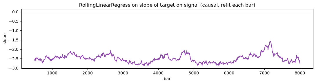
If the model is itself a causal streaming estimator, walk-forward fitting is
already built in and no pairing step is needed. RollingLinearRegression refits a
trailing regression at every bar, so regressing the target on a feature gives a
causal, always-out-of-sample slope directly. forecast_pairs earns its place with
batch learners (trees, boosting, a scaler fit once) that you cannot refit every
bar and must hand a fixed training matrix.
# a causal rolling fit of the target on the signal; column 0 is the slope
roll = np.asarray(RollingLinearRegression(500)(y, sig))
fig, ax = plt.subplots(figsize=(11, 3))
ax.plot(roll[:, 0], color="#8e44ad")
ax.axhline(0, color="k", lw=0.6)
ax.set(title="RollingLinearRegression slope of target on signal (causal, refit each bar)",
       xlabel="bar", ylabel="slope")
fig.tight_layout()
print("the rolling slope stays negative: the fade edge is stable in-sample")
the rolling slope stays negative: the fade edge is stable in-sample
Time-based horizons#
count= shifts by a number of events, which is what a regular bar grid wants. On an
irregular feed, where events do not tick evenly, use duration= to shift by
wall-time instead; internally it uses Delay, the time-based counterpart of Lag,
and needs an index on both X and y. On a regular grid the two agree.
idx = np.cumsum(rng.integers(1, 4, size=n)).astype(np.int64)   # irregular timestamps
Xd, yd, ad = forecast_pairs((sig, idx), (y, idx), duration=h * 2, dropna=True)
print(f"duration-mode pairs: {len(Xd)} rows, aligned by wall-time on an irregular index")
duration-mode pairs: 7995 rows, aligned by wall-time on an irregular index