Bars from ticks: bucketing and aggregations#
Resample condenses a tick stream into fixed bars. Each bar is causal: its value depends only on ticks already seen inside it, never on future ones. A bucket is emitted only once a later timestamp proves it complete; the trailing partial bucket is flushed at end of input.
Two bucketing modes are available. freq=W places bar boundaries on a fixed grid over the index, giving bars of equal index width. count=N closes a bar every N arrivals regardless of their timestamps, giving bars with a fixed number of ticks. Both modes support the same string aggregations, fill= for empty buckets, datetime indexes, and label=/origin= for boundary placement.
import numpy as np
import pandas as pd
import matplotlib.pyplot as plt
from screamer import Resample, to_pandas

rng = np.random.default_rng(42)
n = 80

# Irregular integer timestamps: each tick lands 1-2 units after the last.
timestamps = np.cumsum(rng.integers(1, 3, size=n)).astype(np.int64)

# Mid-price: a slow random walk around 100.
price = 100.0 + np.cumsum(rng.standard_normal(n) * 0.3)

# Trade size: heavy-tailed, always positive.
volume = rng.exponential(scale=50.0, size=n)

# Signed volume: + = buyer-initiated, - = seller-initiated.
signed_volume = volume * rng.choice([-1.0, 1.0], size=n)

# Bar width in index units.
BAR = 20

pd.DataFrame({
    "timestamp":     timestamps[:6],
    "price":         price[:6].round(3),
    "volume":        volume[:6].round(1),
    "signed_volume": signed_volume[:6].round(1),
}).set_index("timestamp")
| price | volume | signed_volume | |
|---|---|---|---|
| timestamp | |||
| 1 | 100.223 | 6.2 | 6.2 |
| 3 | 100.386 | 20.0 | -20.0 |
| 5 | 100.186 | 3.5 | -3.5 |
| 6 | 100.256 | 45.8 | -45.8 |
| 7 | 100.291 | 48.6 | -48.6 |
| 9 | 100.357 | 14.7 | -14.7 |
Mean bars with freq=#
freq=W closes a bar every W units of the index. Boundaries are anchored at
origin (default 0): bar n covers [origin + n*W, origin + (n+1)*W). Bars
have equal index width but a variable number of ticks.
Resample returns a (values, index) tuple. With a 1-D input and a scalar
string agg such as "mean", values is a 1-D array and index holds each
bar's label.
bars = Resample(freq=BAR, agg="mean")(price, timestamps)

values, index = bars
print("bar labels:", index)
print("bar means: ", values.round(3))
bar labels: [  0  20  40  60  80 100 120]
bar means:  [100.582 100.426 100.325  99.878  98.867  97.528  97.366]
OHLCV candles#
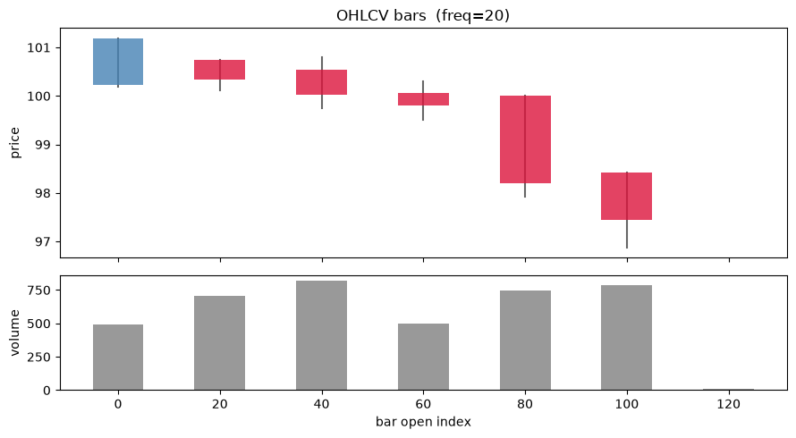
Pass a two-column [price, volume] array and agg="ohlcv". Each bar yields
five positional columns in documented order:
open(0), high(1), low(2), close(3), volume(4).
Use the free helper to_pandas(values, index, columns=[...]) to attach column
names once.
ohlcv_bars = Resample(freq=BAR, agg="ohlcv")(
    np.column_stack([price, volume]), timestamps)

OHLCV_COLS = ["open", "high", "low", "close", "volume"]
df_ohlcv = to_pandas(ohlcv_bars[0], ohlcv_bars[1], columns=OHLCV_COLS)
df_ohlcv.index.name = "bar_open"
df_ohlcv.round(3)
| open | high | low | close | volume | |
|---|---|---|---|---|---|
| bar_open | |||||
| 0 | 100.223 | 101.185 | 100.186 | 101.185 | 493.751 |
| 20 | 100.748 | 100.748 | 100.111 | 100.335 | 706.765 |
| 40 | 100.549 | 100.801 | 99.745 | 100.016 | 818.624 |
| 60 | 100.063 | 100.295 | 99.514 | 99.802 | 496.959 |
| 80 | 100.001 | 100.001 | 97.919 | 98.202 | 746.708 |
| 100 | 98.423 | 98.423 | 96.881 | 97.438 | 785.694 |
| 120 | 97.366 | 97.366 | 97.366 | 97.366 | 9.885 |
ohlcv_vals, ohlcv_idx = ohlcv_bars

fig, (ax_price, ax_vol) = plt.subplots(
    2, 1, figsize=(9, 5), sharex=True,
    gridspec_kw={"height_ratios": [2, 1]},
)

for t, row in zip(ohlcv_idx, ohlcv_vals):
    o, h, l, c = row[:4]
    color = "steelblue" if c >= o else "crimson"
    ax_price.plot([t, t], [l, h], color="0.4", lw=1.5, zorder=1)
    ax_price.bar(t, c - o, bottom=o, width=BAR * 0.5,
                 color=color, alpha=0.8, zorder=2)

ax_price.set_ylabel("price")
ax_price.set_title(f"OHLCV bars  (freq={BAR})")

ax_vol.bar(ohlcv_idx, ohlcv_vals[:, 4], width=BAR * 0.5, color="0.6")
ax_vol.set_ylabel("volume")
ax_vol.set_xlabel("bar open index")
plt.tight_layout()
Buyer- vs seller-initiated volume: ohlcv2#
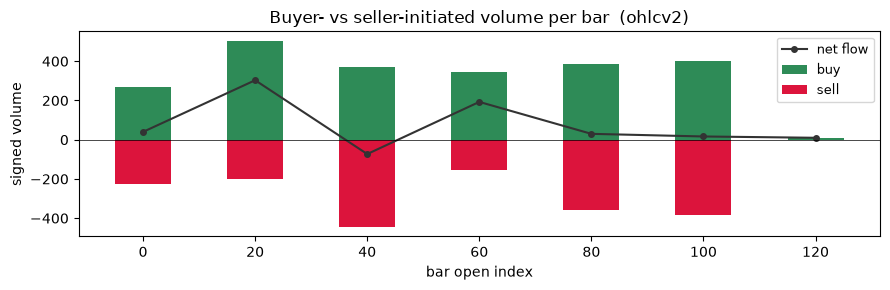
agg="ohlcv2" expects a [price, signed_volume] input (positive = buyer,
negative = seller). Columns are positional:
open(0), high(1), low(2), close(3), buy_vol(4), sell_vol(5).
ohlcv2_vals, ohlcv2_idx = Resample(freq=BAR, agg="ohlcv2")(
    np.column_stack([price, signed_volume]), timestamps)

OHLCV2_COLS = ("open", "high", "low", "close", "buy_vol", "sell_vol")
net_flow = ohlcv2_vals[:, 4] - ohlcv2_vals[:, 5]

fig, ax = plt.subplots(figsize=(9, 3))
ax.bar(ohlcv2_idx,  ohlcv2_vals[:, 4],  width=BAR * 0.5, color="seagreen", label="buy")
ax.bar(ohlcv2_idx, -ohlcv2_vals[:, 5], width=BAR * 0.5, color="crimson",  label="sell")
ax.plot(ohlcv2_idx, net_flow, color="0.2", lw=1.5, marker="o", ms=4, label="net flow")
ax.axhline(0, color="k", lw=0.5)
ax.set_xlabel("bar open index")
ax.set_ylabel("signed volume")
ax.set_title("Buyer- vs seller-initiated volume per bar  (ohlcv2)")
ax.legend(fontsize=9)
plt.tight_layout()
freq= vs count=: the gap test#
The two bucketing modes measure along different axes.
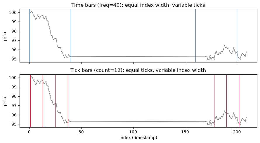
freq=Wplaces boundaries on a fixed grid over the index. A bar with no ticks in its window is an empty bucket.count=Nplaces a boundary everyNarrivals, ignoring the index values. An empty bucket cannot arise.
The stream below has a 130-unit hole after tick 40. freq=40 produces a bar
that straddles the hole with few ticks (and possibly empty bars inside it).
count=12 walks straight across without noticing.
rng2 = np.random.default_rng(7)
n2 = 80

# Dense clock with a 130-unit hole after tick 40.
gaps = np.ones(n2)
gaps[40] = 130
ts2 = np.cumsum(gaps).astype(np.int64)
p2  = 100.0 + np.cumsum(rng2.standard_normal(n2) * 0.3)

print(f"{n2} ticks spanning index {ts2[0]}..{ts2[-1]}")
print(f"hole: {ts2[39]} -> {ts2[40]}")
80 ticks spanning index 1..209
hole: 40 -> 170
EVERY = 40
COUNT = 12

time_mean  = Resample(freq=EVERY,  agg="mean")(p2, ts2)
time_count = Resample(freq=EVERY,  agg="count")(p2, ts2)
tick_mean  = Resample(count=COUNT, agg="mean")(p2, ts2)
tick_count = Resample(count=COUNT, agg="count")(p2, ts2)

print("=== freq= bars (ticks per bar varies) ===")
print(pd.DataFrame({
    "mean":    time_mean[0].round(3),
    "n_ticks": time_count[0].astype(int),
}, index=pd.Index(time_mean[1], name="bar_open")).to_string())

print("\n=== count= bars (index span varies) ===")
first_tick = tick_mean[1]
last_tick  = Resample(count=COUNT, agg="mean", label="right")(p2, ts2)[1]
print(pd.DataFrame({
    "mean":      tick_mean[0].round(3),
    "n_ticks":   tick_count[0].astype(int),
    "last_tick": last_tick,
    "span":      last_tick - first_tick,
}, index=pd.Index(first_tick, name="first_tick")).to_string())
=== freq= bars (ticks per bar varies) ===
            mean  n_ticks
bar_open
0         97.856       39
40        95.258        1
160       95.647       30
200       95.393       10

=== count= bars (index span varies) ===
              mean  n_ticks  last_tick  span
first_tick
1           99.663       12         12    11
13          98.518       12         24    11
25          96.020       12         36    11
37          95.198       12        177   140
178         95.752       12        189    11
190         95.848       12        201    11
202         95.373        8        209     7
fig, (ax_t, ax_c) = plt.subplots(2, 1, sharex=True, figsize=(9, 5))

for ax in (ax_t, ax_c):
    ax.plot(ts2, p2, color="0.5", lw=0.9, marker=".", ms=3)
    ax.set_ylabel("price")

for x in time_mean[1]:
    ax_t.axvline(x, color="steelblue", lw=1.0)
ax_t.set_title(f"Time bars (freq={EVERY}): equal index width, variable ticks")

for x in first_tick:
    ax_c.axvline(x, color="crimson", lw=1.0)
ax_c.set_title(f"Tick bars (count={COUNT}): equal ticks, variable index width")
ax_c.set_xlabel("index (timestamp)")

plt.tight_layout()
Empty bars and fill=#
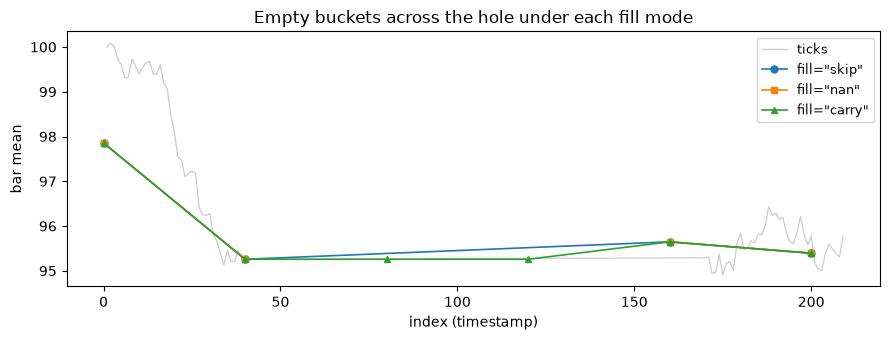
The 130-unit hole is wider than EVERY=40, so one or more intervals on the
grid contain no ticks. fill= controls what Resample emits for those empty
internal buckets:
"skip"(default): emit no row."nan": emit an all-NaN row at the empty bucket's label."carry": repeat the previous bar's values verbatim.
Only buckets between two events are filled. Buckets before the first tick or after the last are not synthesized.
fill= is meaningful only with freq=. Under count=, every bar holds
exactly N events by definition, so an empty bar cannot arise.
modes = ["skip", "nan", "carry"]
frames = {}
for mode in modes:
    b = Resample(freq=EVERY, agg="mean", fill=mode)(p2, ts2)
    frames[mode] = pd.Series(b[0], index=b[1])

# Align on the union of labels to make the gap visible.
pd.DataFrame(frames).round(3)
| skip | nan | carry | |
|---|---|---|---|
| 0 | 97.856 | 97.856 | 97.856 |
| 40 | 95.258 | 95.258 | 95.258 |
| 80 | NaN | NaN | 95.258 |
| 120 | NaN | NaN | 95.258 |
| 160 | 95.647 | 95.647 | 95.647 |
| 200 | 95.393 | 95.393 | 95.393 |
fig, ax = plt.subplots(figsize=(9, 3.5))

ax.plot(ts2, p2, color="0.8", lw=0.9, label="ticks")
for mode, marker in zip(modes, ["o", "s", "^"]):
    s = frames[mode]
    ax.plot(s.index, s.values, marker=marker, ms=5, lw=1.2, label=f'fill="{mode}"')

ax.set_xlabel("index (timestamp)")
ax.set_ylabel("bar mean")
ax.set_title("Empty buckets across the hole under each fill mode")
ax.legend(fontsize=9)
plt.tight_layout()
Datetime indexes#
Pass a NumPy datetime64 array as the index and a pandas offset string as
freq=. Resample infers the datetime context from the index dtype and
aligns bucket boundaries on calendar units.
The returned index is an integer array of nanoseconds since the Unix epoch
(the internal datetime64 representation). Convert it with
pd.to_datetime(index) to get a DatetimeIndex.
dt_index = pd.date_range("2023-01-01", periods=100, freq="1min").values  # datetime64[ns]
rng3  = np.random.default_rng(99)
p3    = 100.0 + np.cumsum(rng3.standard_normal(100) * 0.3)
vol3  = rng3.exponential(scale=50.0, size=100)

dt_bars = Resample(freq="5min", agg="ohlcv")(np.column_stack([p3, vol3]), dt_index)

to_pandas(
    dt_bars[0],
    pd.to_datetime(dt_bars[1]),
    columns=["open", "high", "low", "close", "volume"],
).round(3)
| open | high | low | close | volume | |
|---|---|---|---|---|---|
| 1970-01-20 08:35:31.200 | 100.025 | 100.106 | 99.579 | 99.579 | 152.596 |
| 1970-01-20 08:35:31.500 | 100.085 | 100.085 | 99.454 | 99.734 | 217.597 |
| 1970-01-20 08:35:31.800 | 99.936 | 100.755 | 99.936 | 100.755 | 257.470 |
| 1970-01-20 08:35:32.100 | 101.036 | 101.036 | 100.737 | 100.737 | 256.422 |
| 1970-01-20 08:35:32.400 | 100.954 | 101.231 | 100.848 | 101.231 | 161.502 |
| 1970-01-20 08:35:32.700 | 100.776 | 100.974 | 100.518 | 100.950 | 236.696 |
| 1970-01-20 08:35:33.000 | 101.239 | 101.846 | 101.239 | 101.846 | 279.968 |
| 1970-01-20 08:35:33.300 | 102.053 | 102.308 | 101.581 | 102.308 | 279.185 |
| 1970-01-20 08:35:33.600 | 102.187 | 102.855 | 102.187 | 102.855 | 235.304 |
| 1970-01-20 08:35:33.900 | 103.364 | 103.710 | 103.248 | 103.613 | 363.152 |
| 1970-01-20 08:35:34.200 | 103.616 | 103.842 | 103.492 | 103.754 | 309.860 |
| 1970-01-20 08:35:34.500 | 103.858 | 103.858 | 102.598 | 102.598 | 366.394 |
| 1970-01-20 08:35:34.800 | 102.396 | 102.993 | 102.396 | 102.993 | 354.380 |
| 1970-01-20 08:35:35.100 | 103.097 | 103.097 | 102.259 | 102.259 | 319.916 |
| 1970-01-20 08:35:35.400 | 102.869 | 104.031 | 102.869 | 104.031 | 138.739 |
| 1970-01-20 08:35:35.700 | 103.741 | 103.741 | 103.098 | 103.098 | 273.438 |
| 1970-01-20 08:35:36.000 | 103.074 | 103.109 | 102.887 | 102.892 | 244.679 |
| 1970-01-20 08:35:36.300 | 102.520 | 103.344 | 102.520 | 103.141 | 234.265 |
| 1970-01-20 08:35:36.600 | 103.075 | 103.652 | 103.075 | 103.652 | 391.148 |
| 1970-01-20 08:35:36.900 | 103.391 | 103.415 | 103.170 | 103.232 | 303.300 |
label= and origin=#
By default each bar is labelled by the left edge of its bucket (label="left").
label="right" shifts the label to the right edge instead. The values are
identical; only the index changes.
origin= shifts the grid anchor. With origin=5 and freq=20 the grid is
..., -15, 5, 25, 45, ... instead of ..., 0, 20, 40, ....
left_bars   = Resample(freq=BAR, agg="mean", label="left")(price, timestamps)
right_bars  = Resample(freq=BAR, agg="mean", label="right")(price, timestamps)
origin_bars = Resample(freq=BAR, agg="mean", origin=5)(price, timestamps)

print("label=left  index:", left_bars[1])
print("label=right index:", right_bars[1])
print("origin=5    index:", origin_bars[1])
label=left  index: [  0  20  40  60  80 100 120]
label=right index: [ 20  40  60  80 100 120 140]
origin=5    index: [-15   5  25  45  65  85 105]