Pipelines

A Pipeline wires functions and stream operators into a reusable computation you define once and run either on stored arrays or live, event by event. Run it over whole arrays in one pass, or feed it events one at a time as they arrive; both paths give identical results.

The example is a smoothed spread over two price feeds. The concepts behind the pipeline are in Pipelines.

import numpy as np
import matplotlib.pyplot as plt
from screamer import Input, Pipeline, RollingMean, Sub
from screamer import CombineLatest

Building the pipeline

Input(name) creates a named source. Applying stream operators and functions to those nodes builds more nodes: CombineLatest aligns the two feeds into one two-column stream, Sub() takes their difference, and RollingMean(20) smooths it. Building the pipeline only records structure; nothing runs until you call it. Compiling it into a Pipeline names which nodes are inputs and which are outputs.

a, b = Input("a"), Input("b")

aligned = CombineLatest()(a, b)    # align the two feeds -> a node
spread  = Sub()(aligned)           # difference          -> a node
signal  = RollingMean(20)(spread)  # smooth              -> a node

pipe = Pipeline(inputs=[a, b], outputs=[signal])

Inspecting the pipeline

print(pipe) shows the pipeline as an indented tree, rooted at each output and descending to the inputs, with each node's parameters in its label. This requires no optional dependencies, so it works in any environment. Each node also carries an id (#2); a node shared by several consumers is printed once and then referenced by that id.

print(pipe)

Pipeline(2 input(s), 1 output(s), align_outputs=True)
out[0] = RollingMean(window_size=20)  #4
   └─ Sub()  #3
      └─ CombineLatest(emit='when_all')  #2
         ├─ a  #0 (input)
         └─ b  #1 (input)

The same graph is available as a Graphviz DOT string via pipe.to_dot(), which you can feed to any DOT renderer.

print(pipe.to_dot())

digraph screamer_dag {
  rankdir=LR;
  node [fontname="monospace"];
  n0 [label="a", shape=ellipse, style=filled, fillcolor="#e8f0fe"];
  n1 [label="b", shape=ellipse, style=filled, fillcolor="#e8f0fe"];
  n2 [label="CombineLatest(emit='when_all')", shape=box, style="rounded,filled", fillcolor="#fff3e0"];
  n3 [label="Sub()", shape=box, style=filled, fillcolor="#f5f5f5"];
  n4 [label="RollingMean(window_size=20)", shape=box, style=filled, fillcolor="#f5f5f5", penwidth=2, color="#1a73e8"];
  n0 -> n2;
  n1 -> n2;
  n2 -> n3;
  n3 -> n4;
}

In a notebook, displaying the pipe object directly renders that diagram inline.

pipe.to_graphviz()

Running it: batch and live

pipe(*feeds) runs the whole pipeline over stored arrays in one pass. Pass generators of (value, index) pairs instead of arrays to run event by event: pipe(gen_a, gen_b) returns an iterator of (value, index) events. Each feed is a (values, index) pair.

rng = np.random.default_rng(0)
n = 200
index = np.arange(1, n + 1, dtype=np.int64)
fa = (100 + np.cumsum(rng.standard_normal(n)), index)   # two feeds on the
fb = (100 + np.cumsum(rng.standard_normal(n)), index)   # same timeline

batch_v, batch_idx = pipe(fa, fb)          # whole arrays in

# Event by event via generators
gen_a = ((v, k) for v, k in zip(fa[0], fa[1]))
gen_b = ((v, k) for v, k in zip(fb[0], fb[1]))
events = list(pipe(gen_a, gen_b))
live_v   = np.array([e[0] for e in events])
live_idx = np.array([e[1] for e in events])

import pandas as pd
m = ~np.isnan(batch_v)
pd.DataFrame({"batch": batch_v[m][:5], "live": live_v[m][:5]},
             index=batch_idx[m][:5]).rename_axis("index")

	batch	live
index
20	-0.025896	-0.025896
21	-0.360765	-0.360765
22	-0.550543	-0.550543
23	-0.853429	-0.853429
24	-1.141419	-1.141419

Multiple outputs

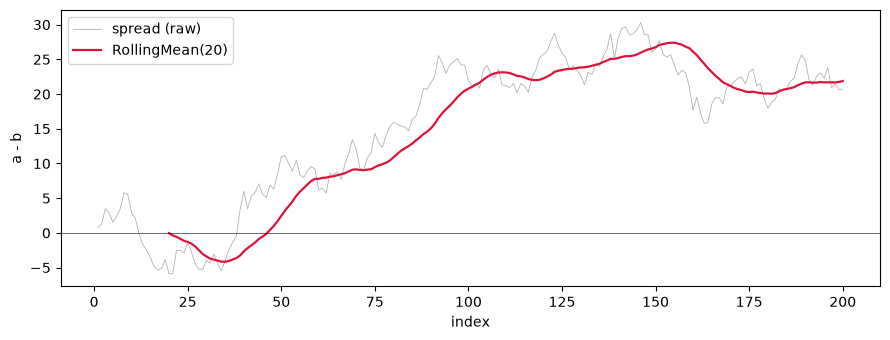
A pipeline can expose more than one output. Adding spread alongside signal gives back the raw difference and its smoothed version together, each as its own (values, index) pair. With align_outputs=True (the default), all outputs are co-indexed onto a shared sorted axis, so every pair has the same length and outputs can be compared sample for sample. Set align_outputs=False to get independent per-output streams whose lengths may differ.

dag2 = Pipeline(inputs=[a, b], outputs=[spread, signal])
(raw_v, raw_idx), (sig_v, sig_idx) = dag2(fa, fb)

fig, ax = plt.subplots(figsize=(9, 3.5))
ax.plot(raw_idx, raw_v, lw=0.6, color="0.7", label="spread (raw)")
ax.plot(sig_idx, sig_v, lw=1.6, color="crimson", label="RollingMean(20)")
ax.axhline(0, color="k", lw=0.4)
ax.set_xlabel("index")
ax.set_ylabel("a - b")
ax.legend(loc="upper left")
plt.tight_layout()

Saving and reloading as JSON

pipe.to_json() serializes the whole pipeline, input names, every node with its parameters, the outputs, and align_outputs, into readable JSON you can write to a config file. Pipeline.from_json(text) rebuilds a runnable pipeline. (to_dict / from_dict do the same with a plain dict.)

import json

config = pipe.to_json()
print(json.dumps(json.loads(config), indent=2))

restored = Pipeline.from_json(config)
restored_v, _ = restored(fa, fb)

{
  "screamer_dag": 1,
  "inputs": [
    "a",
    "b"
  ],
  "align_outputs": true,
  "nodes": [
    {
      "id": 0,
      "kind": "input",
      "name": "a"
    },
    {
      "id": 1,
      "kind": "input",
      "name": "b"
    },
    {
      "id": 2,
      "kind": "operator",
      "op": "CombineLatest",
      "params": {
        "emit": "when_all"
      },
      "in": [
        0,
        1
      ]
    },
    {
      "id": 3,
      "kind": "functor",
      "cls": "Sub",
      "params": {},
      "in": [
        2
      ]
    },
    {
      "id": 4,
      "kind": "functor",
      "cls": "RollingMean",
      "params": {
        "window_size": 20
      },
      "in": [
        3
      ]
    }
  ],
  "outputs": [
    4
  ]
}