Custom and multi-column bars

The built-in string aggregations ("ohlcv", "mean", etc.) cover the most common bar statistics. When you need something different, any screamer functor can serve as the reducer: Resample calls it with reset() at each bar boundary and treats its final output as the bar's value.

For multi-column bars, run one Resample per statistic over the same clock and bar width, then align the results with CombineLatest. Wrapping the whole structure in a Pipeline lets you define the bar schema once and bind new data at call time.

import numpy as np
import pandas as pd
import matplotlib.pyplot as plt
from matplotlib.gridspec import GridSpec
from screamer import (
    Resample, CombineLatest, Input, Pipeline,
    ExpandingSkew, ExpandingSlope, ExpandingStd, ExpandingSum,
    First, Last, ExpandingMax, ExpandingMin,
    PosPart, NegPart,
)

rng = np.random.default_rng(42)
n = 80

# Integer clock: each tick lands 1-2 units after the last.
timestamps = np.cumsum(rng.integers(1, 3, size=n)).astype(np.int64)

# Mid-price: a slow random walk around 100.
price = 100.0 + np.cumsum(rng.standard_normal(n) * 0.3)

# Signed volume: positive = buyer-initiated, negative = seller-initiated.
volume = rng.exponential(scale=50.0, size=n)
signed_volume = volume * rng.choice([-1.0, 1.0], size=n)

# Bar width in index units.
BAR = 20

A single functor as the bar reducer

Pass any screamer functor as agg=. The functor is reset() at each bar boundary, fed every tick in the bar in order, and its final output becomes that bar's value. The statistic is therefore computed causally from the ticks in the bar and nothing else.

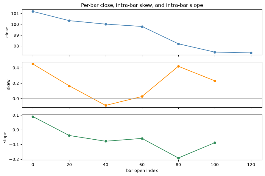
ExpandingSkew() accumulates the first three central moments and returns the bias-corrected skewness coefficient at the bar close. Bars with fewer than three ticks yield NaN.

skew_bars = Resample(freq=BAR, agg=ExpandingSkew())(price, timestamps)

values, index = skew_bars
print("bar labels:    ", index)
print("intra-bar skew:", values.round(4))

bar labels:     [  0  20  40  60  80 100 120]
intra-bar skew: [ 0.449   0.1656 -0.0889  0.027   0.419   0.2307     nan]

Several statistics via CombineLatest composition

Run one Resample per statistic over the same clock and bar width. Because all share the same freq=, they close on the same grid. CombineLatest merges the individual (values, index) tuples into a single multi-column result.

ExpandingSlope() fits a least-squares line to the tick positions within the bar and returns the slope at close. A positive slope means price trended up inside the bar.

slope_bars  = Resample(freq=BAR, agg=ExpandingSlope())(price, timestamps)

# CombineLatest aligns two (values, index) tuples onto a shared grid.
combined = CombineLatest()(skew_bars, slope_bars)
combined_vals, combined_idx = combined

pd.DataFrame(
    combined_vals,
    index=pd.Index(combined_idx, name="bar_open"),
    columns=["skew", "slope"],
).round(4)

	skew	slope
bar_open
0	0.4490	0.0900
20	0.1656	-0.0389
40	-0.0889	-0.0779
60	0.0270	-0.0588
80	0.4190	-0.1917
100	0.2307	-0.0882
120	NaN	NaN

close = Resample(freq=BAR, agg="last")(price, timestamps)

fig, axes = plt.subplots(3, 1, figsize=(9, 6), sharex=True)

axes[0].plot(close[1], close[0], marker="o", ms=5, color="steelblue")
axes[0].set_ylabel("close")
axes[0].set_title("Per-bar close, intra-bar skew, and intra-bar slope")

axes[1].plot(combined_idx, combined_vals[:, 0], marker="o", ms=5, color="darkorange")
axes[1].axhline(0, color="0.6", lw=0.6)
axes[1].set_ylabel("skew")

axes[2].plot(combined_idx, combined_vals[:, 1], marker="o", ms=5, color="seagreen")
axes[2].axhline(0, color="0.6", lw=0.6)
axes[2].set_ylabel("slope")
axes[2].set_xlabel("bar open index")

plt.tight_layout()

Multi-column OHLC + buy/sell bars in a Pipeline

A Pipeline lets you define the bar structure once and bind data at call time. Input nodes are named placeholders; applying a functor to one builds an expression, not a computation.

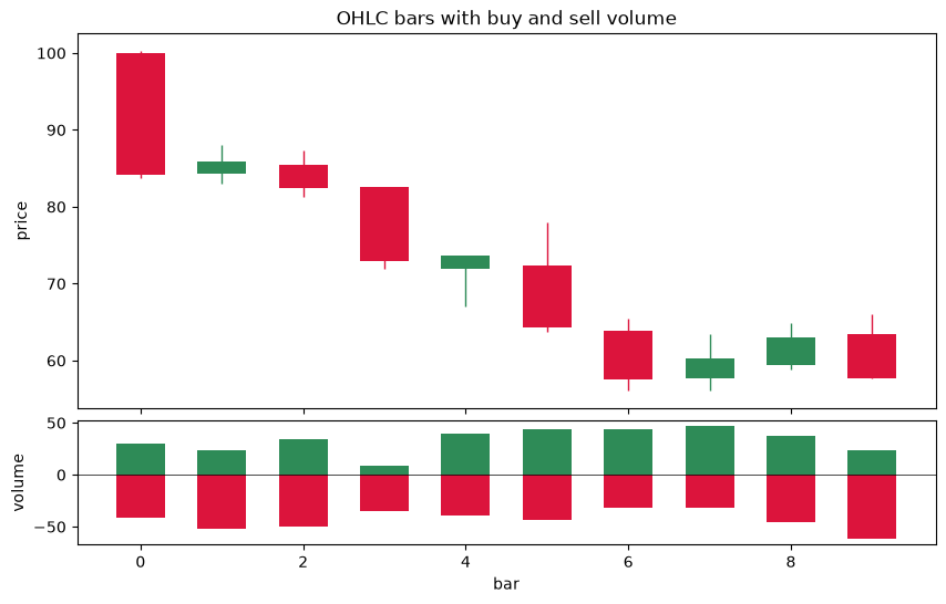
PosPart and NegPart decompose signed volume: every real number satisfies x = PosPart(x) - NegPart(x), with both parts non-negative. Summing each part over a bar splits total traded volume into buyer- and seller-initiated halves.

Every Resample shares the same freq= and clock, so all columns close on the same bar boundaries and cannot drift relative to each other.

rng2 = np.random.default_rng(7)
n2   = 400
BAR2 = 40

t_arr     = np.arange(n2, dtype=np.int64)
price_arr = 100.0 + np.cumsum(rng2.normal(size=n2))
vol_arr   = rng2.normal(size=n2) * rng2.integers(1, 5, size=n2)

# Declare Input placeholders (no data bound yet).
price_in, vol_in = Input("price"), Input("vol")

# Build one node per column.
open_b  = Resample(freq=BAR2, agg=First())(price_in)
high_b  = Resample(freq=BAR2, agg=ExpandingMax())(price_in)
low_b   = Resample(freq=BAR2, agg=ExpandingMin())(price_in)
close_b = Resample(freq=BAR2, agg=Last())(price_in)
buy_b   = Resample(freq=BAR2, agg=ExpandingSum())(PosPart()(vol_in))
sell_b  = Resample(freq=BAR2, agg=ExpandingSum())(NegPart()(vol_in))

# Align all six columns onto one shared bar grid.
bars_node = CombineLatest()(open_b, high_b, low_b, close_b, buy_b, sell_b)
COLUMNS = ["open", "high", "low", "close", "buy", "sell"]

pipe = Pipeline([price_in, vol_in], [bars_node])

# Bind data at call time.
ohlcv, ohlcv_idx = pipe(
    price=(price_arr, t_arr),
    vol=(vol_arr, t_arr),
)

pd.DataFrame(
    ohlcv.round(2),
    index=pd.Index(ohlcv_idx.astype(int), name="bar_open"),
    columns=COLUMNS,
)

	open	high	low	close	buy	sell
bar_open
0	100.00	100.30	83.78	84.19	30.14	41.24
40	84.30	88.11	83.03	85.89	23.37	51.61
80	85.46	87.37	81.26	82.43	34.53	49.69
120	82.52	82.52	71.97	72.95	9.15	34.56
160	71.90	73.64	67.07	73.61	39.73	39.35
200	72.36	77.95	63.67	64.33	43.55	43.31
240	63.87	65.47	56.08	57.55	44.23	31.67
280	57.64	63.41	56.11	60.23	47.11	31.38
320	59.46	64.86	58.78	62.94	37.49	46.11
360	63.45	65.97	57.71	57.71	24.12	61.95

o, h, l, c  = ohlcv[:, 0], ohlcv[:, 1], ohlcv[:, 2], ohlcv[:, 3]
buy, sell   = ohlcv[:, 4], ohlcv[:, 5]

fig = plt.figure(figsize=(10, 6))
gs = GridSpec(2, 1, height_ratios=[3, 1], hspace=0.05)
ax1 = fig.add_subplot(gs[0])
ax2 = fig.add_subplot(gs[1], sharex=ax1)

x = np.arange(len(o))
colors = np.where(c >= o, "seagreen", "crimson")
ax1.vlines(x, l, h, color=colors, lw=1)
ax1.bar(x, np.abs(c - o), bottom=np.minimum(o, c), color=colors, width=0.6)
ax1.set_ylabel("price")
ax1.set_title("OHLC bars with buy and sell volume")
ax1.tick_params(labelbottom=False)

ax2.bar(x,  buy,  color="seagreen", width=0.6)
ax2.bar(x, -sell, color="crimson",  width=0.6)
ax2.axhline(0, color="k", lw=0.5)
ax2.set_ylabel("volume")
ax2.set_xlabel("bar")

Text(0.5, 0, 'bar')

Extending the bar

Adding a column means adding one more Resample node and including it in CombineLatest. The rest of the graph is unchanged.

The example below adds realized volatility (rvol): the standard deviation of price ticks within the bar, computed by ExpandingStd(). Note that this is a price dispersion measure, not a traded volume column.

price3, vol3 = Input("price"), Input("vol")
close3 = Resample(freq=BAR2, agg=Last())(price3)
rvol3  = Resample(freq=BAR2, agg=ExpandingStd())(price3)   # price std per bar
flow3  = Resample(freq=BAR2, agg=ExpandingSum())(vol3)

bars3 = CombineLatest()(close3, rvol3, flow3)
COLS3 = ["close", "rvol", "flow"]

out, out_idx = Pipeline([price3, vol3], [bars3])(
    price=(price_arr, t_arr),
    vol=(vol_arr, t_arr),
)

pd.DataFrame(
    out.round(3),
    index=pd.Index(out_idx.astype(int), name="bar_open"),
    columns=COLS3,
)

	close	rvol	flow
bar_open
0	84.193	6.035	-11.095
40	85.887	1.356	-28.248
80	82.429	1.666	-15.154
120	72.953	2.311	-25.410
160	73.608	1.834	0.384
200	64.329	4.412	0.250
240	57.554	2.865	12.557
280	60.235	2.171	15.723
320	62.944	1.552	-8.615
360	57.706	2.038	-37.824