Microstructure III: toxicity, book pressure, and spreads#
The order-flow tape tells you how one-sided trading is; the order book tells you where price is likely to go next and what it costs to trade.
Toxicity runs on the real Deribit BTC-perpetual tape (the six-hour slice under
data/). The book operators need bid and ask quotes, which a trade tape does not
carry, so the book sections use a small illustrative L1 book.
Operators: VPIN, QueueImbalance, MicroPrice, ContOFI, EffectiveSpread,
and RealizedSpread.
import numpy as np
import pandas as pd
import matplotlib.pyplot as plt
from screamer import (VPIN, MicroPrice, ContOFI, EffectiveSpread, RealizedSpread)
from screamer.microstructure import QueueImbalance
Order-flow toxicity: VPIN#
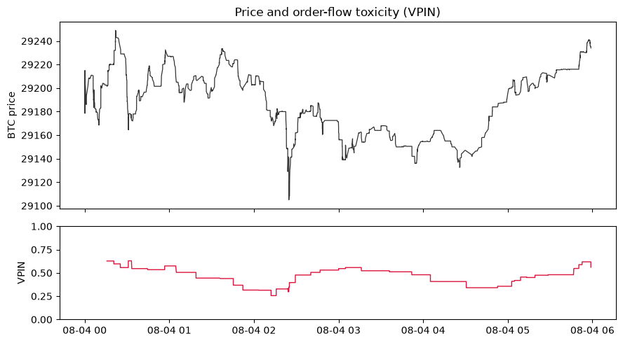
VPIN measures how one-sided flow is over a volume clock: trades are packed
into equal-volume buckets, and VPIN averages the absolute buy-minus-sell
imbalance across the last few buckets, in [0, 1]. A high value marks toxic,
informed flow that often precedes sharp moves. We split each real trade into its
buy or sell leg using the venue's aggressor sign, then run VPIN.
trades = pd.read_csv("data/deribit_btc_perp_6h.csv")
ts = trades["timestamp"].to_numpy(np.int64)
price = trades["price"].to_numpy(np.float64)
signed_vol = trades["volume"].to_numpy(np.float64)     # + buyer, - seller
size = np.abs(signed_vol)

buy_vol = np.where(signed_vol > 0, size, 0.0)
sell_vol = np.where(signed_vol < 0, size, 0.0)

# bucket ~ 1/50 of the session's volume; average toxicity over 10 buckets
bucket = size.sum() / 50
vpin = VPIN(bucket_volume=bucket, n_buckets=10)(buy_vol, sell_vol)

tt = pd.to_datetime(ts, unit="ms")
fig, (a0, a1) = plt.subplots(2, 1, sharex=True, figsize=(9, 5),
                             gridspec_kw={"height_ratios": [2, 1]})
a0.plot(tt, price, color="0.2", lw=0.9)
a0.set_ylabel("BTC price"); a0.set_title("Price and order-flow toxicity (VPIN)")
a1.plot(tt, vpin, color="crimson", lw=1.0); a1.set_ylim(0, 1)
a1.set_ylabel("VPIN")
plt.tight_layout()
Book pressure and fair value#
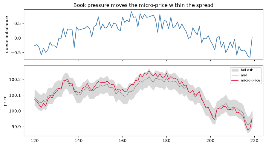
The next operators read the resting order book. A trade tape has no quotes, so the book below is illustrative: a mid that random-walks, a fixed half-spread, and top-of-book sizes driven by a slow latent pressure.
QueueImbalance normalizes the resting sizes to [-1, 1], and MicroPrice
leans the fair value toward the thinner side. In fact the two are the same signal:
the micro-price sits at mid + half_spread * imbalance, so it rides within the
spread exactly as the imbalance shifts.
rng = np.random.default_rng(0)
n = 400
half_spread = 0.05
pressure = np.sin(np.linspace(0, 6 * np.pi, n)) + 0.25 * rng.standard_normal(n)
mid = 100 + np.cumsum(rng.standard_normal(n) * 0.02)
bid, ask = mid - half_spread, mid + half_spread
bid_size = (2 + 1.5 * pressure).clip(0.2) + 0.3 * np.abs(rng.standard_normal(n))
ask_size = (2 - 1.5 * pressure).clip(0.2) + 0.3 * np.abs(rng.standard_normal(n))

imbalance = QueueImbalance()(bid_size, ask_size)
micro = MicroPrice()(bid, ask, bid_size, ask_size)

w = slice(120, 220)                                    # a zoomed window
x = np.arange(n)[w]
fig, (a0, a1) = plt.subplots(2, 1, sharex=True, figsize=(9, 5),
                             gridspec_kw={"height_ratios": [1, 1.4]})
a0.plot(x, imbalance[w], color="steelblue"); a0.axhline(0, color="k", lw=0.5)
a0.set_ylabel("queue imbalance"); a0.set_title("Book pressure moves the micro-price within the spread")
a1.fill_between(x, bid[w], ask[w], color="0.85", label="bid-ask")
a1.plot(x, mid[w], color="0.5", lw=1.0, label="mid")
a1.plot(x, micro[w], color="crimson", lw=1.2, label="micro-price")
a1.set_ylabel("price"); a1.legend(loc="upper right", fontsize=8)
plt.tight_layout()
Order-book flow: ContOFI#
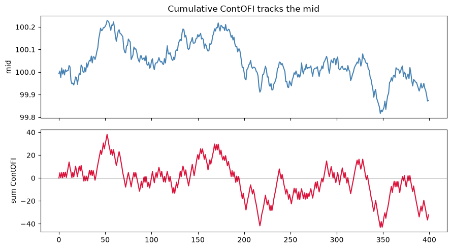
ContOFI is the Cont-Kukanov-Stoikov order-flow imbalance from book events: each
change in the best quotes and their sizes contributes signed depth. Summed, it is
a running measure of net book pressure that tracks the mid.
ofi = ContOFI()(bid, ask, bid_size, ask_size)
cum = np.cumsum(np.nan_to_num(ofi))

fig, (a0, a1) = plt.subplots(2, 1, sharex=True, figsize=(9, 5))
a0.plot(mid, color="steelblue"); a0.set_ylabel("mid"); a0.set_title("Cumulative ContOFI tracks the mid")
a1.plot(cum, color="crimson"); a1.axhline(0, color="k", lw=0.5); a1.set_ylabel("sum ContOFI")
plt.tight_layout()
What a trade really costs: effective and realized spread#
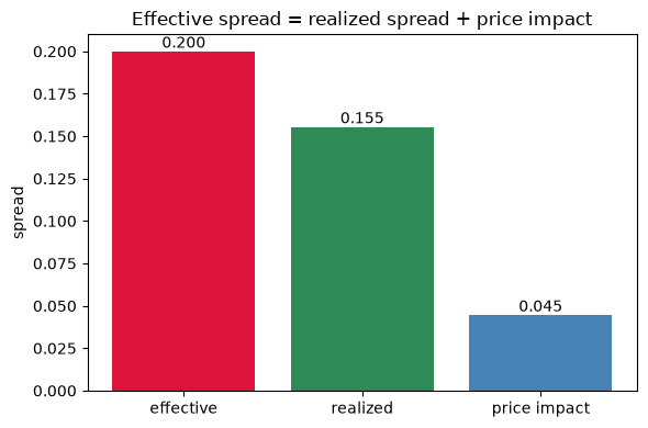
EffectiveSpread is the round-trip cost paid relative to the mid, 2*|price - mid|. RealizedSpread is the part the liquidity provider keeps once the price
has moved, 2*D*(price - mid a few steps later). Their difference is the
price-impact, or adverse-selection, component. Below, informed trades push the
mid in their own direction after they print, so the realized spread sits well
below the effective spread.
rng = np.random.default_rng(1)
n, hs = 3000, 0.10
mid = np.empty(n); mid[0] = 100.0
price = np.empty(n); side = rng.choice([-1.0, 1.0], size=n)
for t in range(n):
    price[t] = mid[t] + side[t] * hs                   # trade at the bid or the offer
    if t + 1 < n:
        mid[t + 1] = mid[t] + rng.standard_normal() * 0.01 + side[t] * 0.02   # adverse drift

eff = EffectiveSpread()(price, mid)
real = RealizedSpread(lag=30)(price, mid)
impact = eff - real

fig, ax = plt.subplots(figsize=(6, 4))
means = [np.nanmean(eff), np.nanmean(real), np.nanmean(impact)]
ax.bar(["effective", "realized", "price impact"], means,
       color=["crimson", "seagreen", "steelblue"])
for i, m in enumerate(means):
    ax.text(i, m, f"{m:.3f}", ha="center", va="bottom")
ax.set_ylabel("spread"); ax.set_title("Effective spread = realized spread + price impact")
plt.tight_layout()