Microstructure I: order flow, trade signs, and imbalance

Trades carry a direction. A buyer lifting the offer pushes price up; a seller hitting the bid pushes it down. Recovering that direction from a raw trade tape, and summing it into order-flow imbalance, is the first step in short-horizon price models.

This notebook runs on a real tape: six hours of Deribit BTC-perpetual trades from 2023-08-04, a committed slice under data/. The volume column is already aggressor-signed (positive is buyer-initiated, negative is seller-initiated), which gives a ground truth to check the classifiers against.

Every operator here is causal: its value at each trade depends only on trades already seen.

import numpy as np
import pandas as pd
import matplotlib.pyplot as plt
from screamer import (TickRuleSign, SignedVolume, OFI, RollingOrderImbalance,
                      BulkVolumeClassifier, HawkesIntensity, Resample, LogReturn)

trades = pd.read_csv("data/deribit_btc_perp_6h.csv")
ts    = trades["timestamp"].to_numpy(np.int64)      # milliseconds since epoch
price = trades["price"].to_numpy(np.float64)
signed_vol = trades["volume"].to_numpy(np.float64)  # + buyer, - seller (venue truth)
size      = np.abs(signed_vol)
true_sign = np.sign(signed_vol)

print(f"{len(trades):,} trades   "
      f"{pd.to_datetime(ts[0], unit='ms')}  ..  {pd.to_datetime(ts[-1], unit='ms')}")
trades.head()

4,093 trades   2023-08-04 00:00:00.068000  ..  2023-08-04 05:58:53.995000

	timestamp	volume	price
0	1691107200068	-10.0	29201.5
1	1691107200068	-590.0	29201.5
2	1691107200090	-190.0	29201.5
3	1691107201710	-800.0	29201.5
4	1691107201793	-790.0	29201.5

Recovering the trade sign from price alone

Most public tapes do not say who was the aggressor. The tick rule infers it from price changes: a trade above the previous price is a buy (+1), below is a sell (-1), and an unchanged price carries the last sign forward. TickRuleSign needs only the price series.

Because this tape also carries the venue's true sign, we can measure how often the tick rule agrees with it.

tick_sign = TickRuleSign()(price)

# Compare only where the tick rule has committed to a sign (skip the leading NaN).
valid = ~np.isnan(tick_sign)
agree = (tick_sign[valid] == true_sign[valid]).mean()
print(f"tick rule agrees with the venue sign on {agree:.1%} of trades")

tick rule agrees with the venue sign on 79.3% of trades

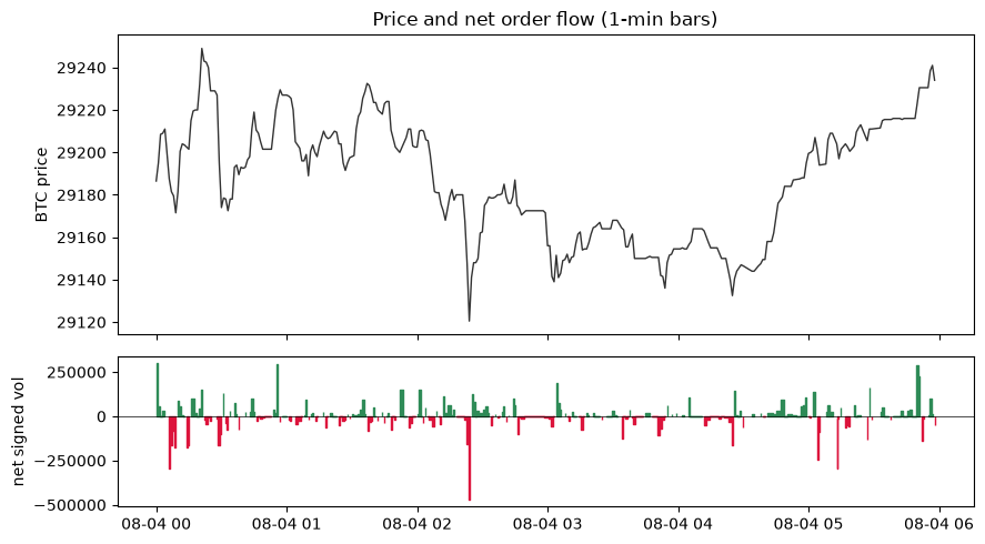
Signed volume and net flow

SignedVolume multiplies a sign by size to give aggressor-signed order flow. Summed over a bar it is the net quantity bought, the raw material of every flow model below. Here we bucket trades into one-minute bars and plot net flow beneath the price.

signed_flow = SignedVolume()(true_sign, size)   # venue-signed order flow per trade

BAR_MS = 60_000                                 # one-minute bars
net_flow = Resample(freq=BAR_MS, agg="sum")(signed_flow, ts)
close    = Resample(freq=BAR_MS, agg="last")(price, ts)
fv, fidx = net_flow
cv, _    = close
bt = pd.to_datetime(fidx, unit="ms")

fig, (a0, a1) = plt.subplots(2, 1, sharex=True, figsize=(9, 5),
                             gridspec_kw={"height_ratios": [2, 1]})
a0.plot(bt, cv, color="0.2", lw=1.0)
a0.set_ylabel("BTC price"); a0.set_title("Price and net order flow (1-min bars)")
a1.fill_between(bt, fv, 0, where=fv >= 0, color="seagreen", step="mid")
a1.fill_between(bt, fv, 0, where=fv < 0,  color="crimson",  step="mid")
a1.axhline(0, color="k", lw=0.5); a1.set_ylabel("net signed vol")
plt.tight_layout()

Order-flow imbalance (OFI)

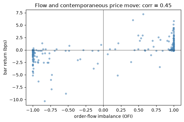
OFI normalizes net flow to [-1, 1] as (buy - sell) / (buy + sell). It is scale-free, so it is comparable across bars and across assets. Resample(agg="ohlcv2") splits each bar into buy and sell volume legs, which feed OFI directly. We then line up each bar's imbalance with its own return.

ohlcv2 = Resample(freq=BAR_MS, agg="ohlcv2")(
    np.column_stack([price, signed_flow]), ts)
cols = ohlcv2[0]
buy_vol, sell_vol = cols[:, 4], cols[:, 5]
open_, close_     = cols[:, 0], cols[:, 3]

ofi     = OFI()(buy_vol, sell_vol)
bar_ret = np.log(close_) - np.log(open_)        # contemporaneous bar return

m = ~np.isnan(ofi)
corr = np.corrcoef(ofi[m], bar_ret[m])[0, 1]
print(f"corr(OFI, bar return) = {corr:.2f}   over {m.sum()} bars")

corr(OFI, bar return) = 0.45   over 319 bars

fig, ax = plt.subplots(figsize=(6, 4))
ax.scatter(ofi[m], 1e4 * bar_ret[m], s=12, alpha=0.5, color="steelblue")
ax.axhline(0, color="k", lw=0.5); ax.axvline(0, color="k", lw=0.5)
ax.set_xlabel("order-flow imbalance (OFI)"); ax.set_ylabel("bar return (bps)")
ax.set_title(f"Flow and contemporaneous price move: corr = {corr:.2f}")
plt.tight_layout()

Persistence and clustering

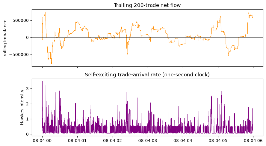
Order flow is autocorrelated: buys tend to follow buys. RollingOrderImbalance tracks the trailing net flow over a fixed number of trades. HawkesIntensity models trading as a self-exciting process on a time clock: each arrival briefly lifts the expected rate of the next, so bursts of activity show up as spikes in the intensity that decay through the quiet that follows.

roll_imb = RollingOrderImbalance(200)(signed_flow)

# Hawkes intensity on a one-second clock: mark each second in which a trade
# printed, so quiet seconds let the intensity decay between bursts (feeding one
# event per trade would saturate to a constant rate).
sec = ((ts - ts[0]) // 1000).astype(int)
event = np.zeros(sec.max() + 1)
event[np.unique(sec)] = 1.0
intensity = HawkesIntensity(decay=0.9, alpha=0.5, mu=0.05)(event)
sec_time = pd.to_datetime(ts[0] + np.arange(len(event)) * 1000, unit="ms")
tt = pd.to_datetime(ts, unit="ms")

fig, (a0, a1) = plt.subplots(2, 1, sharex=True, figsize=(9, 5))
a0.plot(tt, roll_imb, color="darkorange", lw=0.8); a0.axhline(0, color="k", lw=0.5)
a0.set_ylabel("rolling imbalance"); a0.set_title("Trailing 200-trade net flow")
a1.plot(sec_time, intensity, color="purple", lw=0.7)
a1.set_ylabel("Hawkes intensity")
a1.set_title("Self-exciting trade-arrival rate (one-second clock)")
plt.tight_layout()

Bulk Volume Classification

BulkVolumeClassifier estimates the buy-initiated fraction of each bar from its return and trailing volatility alone, with no per-trade signs. It is a bar-level counterpart to the tick rule, and we can check it against the true buy share.

bar_logret   = LogReturn(1)(close_)
buy_fraction = BulkVolumeClassifier(20)(bar_logret)
actual_share = buy_vol / (buy_vol + sell_vol)

mm = ~np.isnan(buy_fraction)
print(f"corr(BVC estimate, actual buy share) = "
      f"{np.corrcoef(buy_fraction[mm], actual_share[mm])[0, 1]:.2f}")

corr(BVC estimate, actual buy share) = 0.50