Backtesting a signal: from indicator to a costed equity curve

BacktestPriceTarget turns a position signal and a price into a mark-to-market equity curve with transaction costs, and backtest_report reads off the statistics. This example builds a trend signal on real Deribit BTC-perpetual bars and backtests it, with and without cost.

import numpy as np
import pandas as pd
import matplotlib.pyplot as plt
from screamer import BacktestPriceTarget, RollingMean, backtest_report, Resample

trades = pd.read_csv("data/deribit_btc_perp_6h.csv")
ts = trades["timestamp"].to_numpy(np.int64)
price = trades["price"].to_numpy(np.float64)
close, idx = Resample(freq=60_000, agg="last")(price, ts)   # one-minute close
t = pd.to_datetime(idx, unit="ms")
print(f"{len(close)} one-minute bars")

319 one-minute bars

A trend signal

A moving-average crossover: hold long when the fast average is above the slow one, short when it is below. np.sign maps that to a position of +1 or -1; the warmup region is flat (0).

fast = RollingMean(5)(close)
slow = RollingMean(30)(close)
signal = np.sign(np.nan_to_num(fast - slow))   # +1 long, -1 short, 0 while warming up

Backtest it, with and without cost

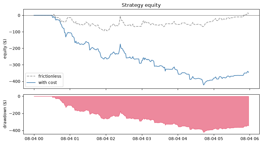
The frictionless run is the raw edge of the signal; the costed run charges a 5 bps spread and a 2 bps fee on every trade. The gap between them is what trading costs eat.

free = BacktestPriceTarget()(signal, close)
costed = BacktestPriceTarget(spread=0.0005, fee=0.0002)(signal, close)
running, summary = backtest_report(costed)      # running columns + summary (no pandas)

eq_f, eq_c = free[:, 0], costed[:, 0]
dd = running["drawdown"]                          # dollar drawdown, from the BacktestReport node

fig, (a0, a1) = plt.subplots(2, 1, sharex=True, figsize=(9, 5),
                             gridspec_kw={"height_ratios": [2, 1]})
a0.plot(t, eq_f, color="0.6", ls="--", label="frictionless")
a0.plot(t, eq_c, color="steelblue", label="with cost")
a0.axhline(0, color="k", lw=0.5); a0.set_ylabel("equity ($)")
a0.set_title("Strategy equity"); a0.legend()
a1.fill_between(t, dd, 0, color="crimson", alpha=0.5); a1.set_ylabel("drawdown ($)")
plt.tight_layout()

The statistics

backtest_report aggregates the engine's [equity, pnl, position, cost] output into the summary every backtest wants.

for name, value in summary.items():             # summary is a plain dict of floats
    print(f"{name:13s} {value:10.4f}")

total_pnl      -346.5605
max_drawdown   -422.5605
total_cost      354.5605
turnover         27.0000
num_trades       15.0000
sharpe           -0.1481

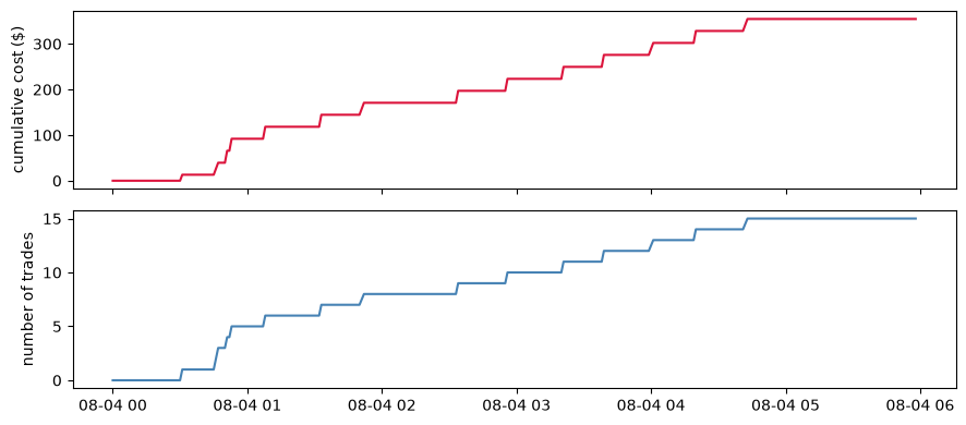
Statistics are running series

Each statistic produced by backtest_report is a causal time series, so you can watch the cost and the trade count accumulate through the session, not just read the final number.

fig, (a0, a1) = plt.subplots(2, 1, sharex=True, figsize=(9, 4))
a0.plot(t, running["cum_cost"], color="crimson"); a0.set_ylabel("cumulative cost ($)")
a1.plot(t, running["trades"], color="steelblue"); a1.set_ylabel("number of trades")
plt.tight_layout()