Microstructure II: price impact and liquidity

Order flow moves price, but by how much per unit traded? That slope is price impact, and its inverse is liquidity. This notebook estimates both from trades alone, on real Deribit BTC- and ETH-perpetual tapes (six-hour slices under data/), and contrasts the two assets. Every operator here is causal.

import numpy as np
import pandas as pd
import matplotlib.pyplot as plt
from screamer import (RollingKyleLambda, EwKyleLambda, AmihudIlliquidity,
                      RollSpread, Propagator, SignedVolume, Resample, LogReturn)


def load_bars(path, bar_ms=60_000):
    """One-minute bars: close, log return, net signed flow, and notional."""
    tr = pd.read_csv(path)
    ts = tr["timestamp"].to_numpy(np.int64)
    price = tr["price"].to_numpy(np.float64)
    sv = tr["volume"].to_numpy(np.float64)             # venue-signed size
    flow = SignedVolume()(np.sign(sv), np.abs(sv))
    cv, idx  = Resample(freq=bar_ms, agg="last")(price, ts)
    netflow  = Resample(freq=bar_ms, agg="sum")(flow, ts)[0]
    notional = Resample(freq=bar_ms, agg="sum")(np.abs(sv) * price, ts)[0]
    return pd.DataFrame({"close": cv, "ret": LogReturn(1)(cv),
                         "flow": netflow, "notional": notional},
                        index=pd.to_datetime(idx, unit="ms"))


btc = load_bars("data/deribit_btc_perp_6h.csv")
eth = load_bars("data/deribit_eth_perp_6h.csv")
print(f"BTC bars: {len(btc)}   ETH bars: {len(eth)}")
btc.head()

BTC bars: 319   ETH bars: 258

	close	ret	flow	notional
2023-08-04 00:00:00	29186.5	NaN	298100.0	4.304829e+10
2023-08-04 00:01:00	29195.0	0.000291	53880.0	2.830672e+09
2023-08-04 00:02:00	29208.5	0.000462	600.0	1.752440e+07
2023-08-04 00:03:00	29209.0	0.000017	30750.0	9.133507e+08
2023-08-04 00:04:00	29211.0	0.000068	12170.0	3.554857e+08

Kyle's lambda: the price-impact slope

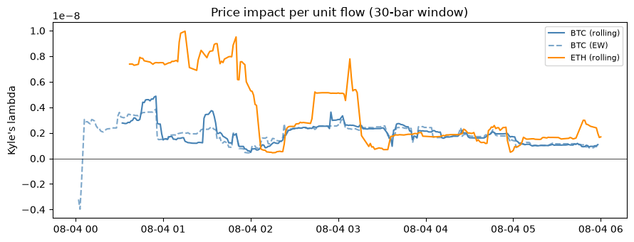
Kyle (1985) models the bar return as r = lambda * flow + noise. The slope lambda is the price move per unit of signed volume: a high lambda means a thin book that is easily moved. RollingKyleLambda regresses return on signed flow over a trailing window; EwKyleLambda does the same with exponential weighting, so it adapts faster. Lambda is quoted per contract, so we read it as liquidity changing over time within an asset rather than comparing the two levels.

W = 30
for df in (btc, eth):
    f, r = df["flow"].to_numpy(), df["ret"].to_numpy()
    df["kyle"]    = RollingKyleLambda(W)(f, r)
    df["kyle_ew"] = EwKyleLambda(float(W))(f, r)

fig, ax = plt.subplots(figsize=(9, 3.5))
ax.plot(btc.index, btc["kyle"],    color="steelblue", label="BTC (rolling)")
ax.plot(btc.index, btc["kyle_ew"], color="steelblue", ls="--", alpha=0.7, label="BTC (EW)")
ax.plot(eth.index, eth["kyle"],    color="darkorange", label="ETH (rolling)")
ax.axhline(0, color="k", lw=0.5)
ax.set_ylabel("Kyle's lambda"); ax.set_title(f"Price impact per unit flow ({W}-bar window)")
ax.legend(fontsize=8); plt.tight_layout()

Amihud illiquidity: cost per dollar traded

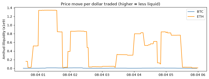
Amihud (2002) measures illiquidity as the average of |return| / notional: how far price moves per dollar of volume. Dividing by notional makes it comparable across assets. AmihudIlliquidity keeps a rolling mean of that ratio.

for df in (btc, eth):
    df["amihud"] = AmihudIlliquidity(W)(df["ret"].to_numpy(), df["notional"].to_numpy())

fig, ax = plt.subplots(figsize=(9, 3.5))
ax.plot(btc.index, 1e9 * btc["amihud"], color="steelblue", label="BTC")
ax.plot(eth.index, 1e9 * eth["amihud"], color="darkorange", label="ETH")
ax.set_ylabel("Amihud illiquidity (x1e9)")
ax.set_title("Price move per dollar traded (higher = less liquid)")
ax.legend(); plt.tight_layout()
print(f"median Amihud   BTC={btc['amihud'].median():.2e}   ETH={eth['amihud'].median():.2e}")

median Amihud   BTC=3.06e-12   ETH=5.28e-10

Roll's effective spread

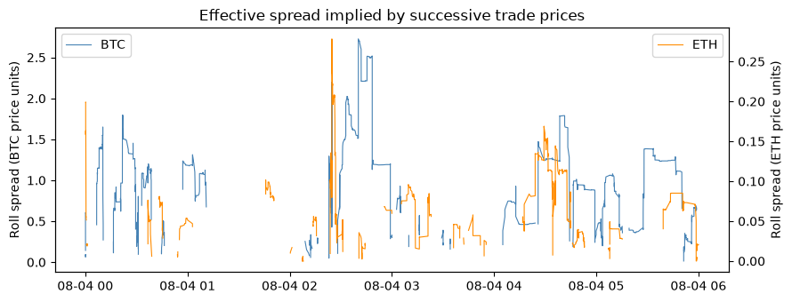
Roll (1984) recovers the effective bid-ask spread from trade prices alone. The bid-ask bounce makes successive trade prices negatively autocovaried, so spread = 2 * sqrt(-cov(dP_t, dP_{t-1})). Because the bounce is a trade-level effect, we run it over a trailing window of trades, not bars. Windows where the serial covariance turns positive (a trending stretch) leave the spread undefined and show as gaps.

fig, ax = plt.subplots(figsize=(9, 3.5))
ax2 = ax.twinx()
for path, name, color, target in [("data/deribit_btc_perp_6h.csv", "BTC", "steelblue", ax),
                                  ("data/deribit_eth_perp_6h.csv", "ETH", "darkorange", ax2)]:
    tr = pd.read_csv(path)
    t = pd.to_datetime(tr["timestamp"], unit="ms")
    spread = RollSpread(100)(tr["price"].to_numpy(np.float64))   # on successive trades
    target.plot(t, spread, color=color, lw=0.8, label=name)
ax.set_ylabel("Roll spread (BTC price units)")
ax2.set_ylabel("Roll spread (ETH price units)")
ax.set_title("Effective spread implied by successive trade prices")
ax.legend(loc="upper left"); ax2.legend(loc="upper right")
plt.tight_layout()

The Bouchaud propagator: impact with memory

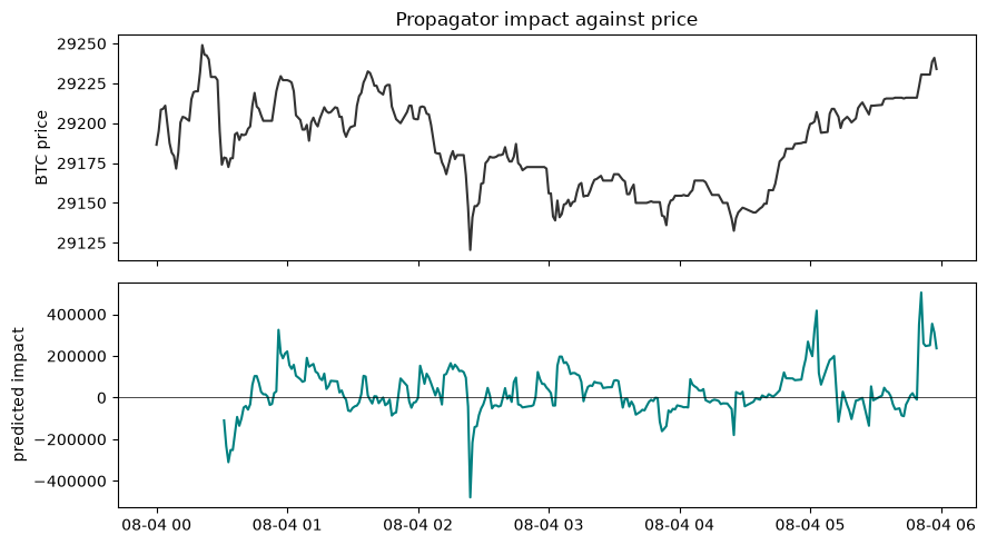
Kyle's lambda treats each trade's impact as instantaneous and permanent. The Bouchaud (2004) propagator instead sums past signed flow through a decaying power-law kernel, so impact builds and then relaxes. Propagator convolves the signed-flow series with that kernel to predict the impact path.

btc["impact"] = Propagator(window=30, g0=1.0, gamma=0.4)(btc["flow"].to_numpy())

fig, (a0, a1) = plt.subplots(2, 1, sharex=True, figsize=(9, 5))
a0.plot(btc.index, btc["close"], color="0.2")
a0.set_ylabel("BTC price"); a0.set_title("Propagator impact against price")
a1.plot(btc.index, btc["impact"], color="teal"); a1.axhline(0, color="k", lw=0.5)
a1.set_ylabel("predicted impact")
plt.tight_layout()