Denoising filters: a comparison

Recovering a slow underlying signal from noisy measurements is one of the most common jobs in a data pipeline. screamer offers several filter families for it, and they make different trade-offs: smoothness, lag (phase delay), robustness to outliers, and compute cost. No single filter wins on every count. Every filter here is causal, using only past and present samples. All window-based filters use a window of 31 so their responsiveness lines up.

import numpy as np
import matplotlib.pyplot as plt
from screamer import (RollingMean, EwMean, RollingMedian, Butter, MovingAverage,
                      RollingPoly1, RollingPoly2, ImpulseClip)

rng = np.random.default_rng(7)
n = 400
t = np.linspace(0, 6 * np.pi, n)
clean = np.sin(t) + 0.35 * np.sin(2.9 * t + 0.6)   # the signal we want back
noisy = clean + 0.30 * rng.standard_normal(n)      # broadband noise

W = 31   # window for the smoothing families


def show(title, curves, faint=()):
    "Plot the noisy signal and the clean reference, with the given filters on top."
    fig, ax = plt.subplots(figsize=(9, 3.2))
    ax.plot(noisy, lw=0.5, color="0.75", label="noisy")
    ax.plot(clean, lw=1.1, color="0.35", ls="--", label="clean signal")
    for label, y in curves.items():
        emphasised = label not in faint
        ax.plot(y, lw=1.8 if emphasised else 1.0, alpha=1.0 if emphasised else 0.55, label=label)
    ax.set_title(title)
    ax.set_xlabel("sample")
    ax.set_ylim(-2.2, 2.2)
    ax.legend(loc="upper right", fontsize=8, ncol=2)
    plt.tight_layout()

Moving average and exponential average

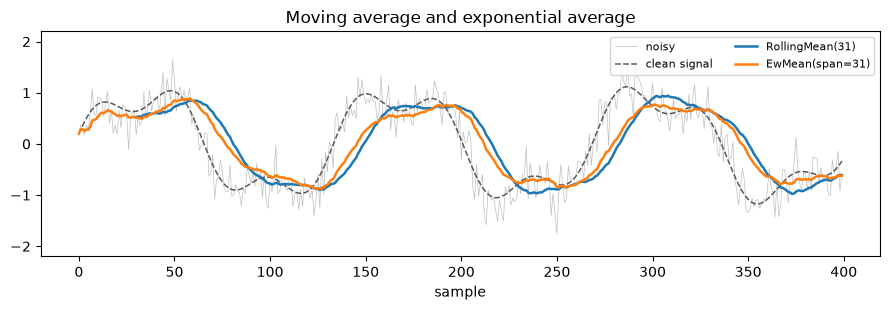
RollingMean averages the last n samples with equal weight. EwMean keeps all history but lets it decay geometrically, so recent samples count more. Both are cheap: RollingMean updates in constant time from a running sum, and EwMean holds a single number with no window buffer. For a given responsiveness, they are the smoothest options available.

The cost is lag and fragility. Equal weighting delays the output by roughly half the window; exponential weighting turns with the data sooner but still trails. Because every sample enters the average, a lone outlier smears into the output as a bump that lasts a full window.

show("Moving average and exponential average", {
    "RollingMean(31)":  RollingMean(W)(noisy),
    "EwMean(span=31)":  EwMean(span=W)(noisy),
})

Median filter

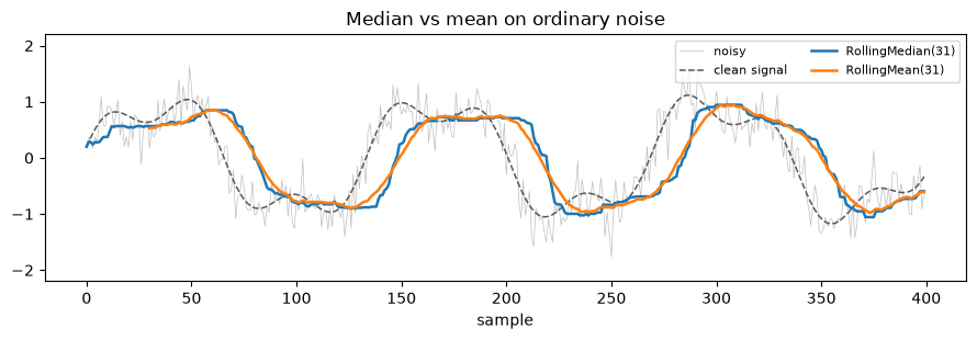
RollingMedian reports the middle value of the window instead of the average. Because a few extreme samples cannot move the middle, it ignores outliers that would pull an average off course and preserves step edges that a mean would round off.

On ordinary noise, though, the mean is hard to beat: averaging cancels zero-mean noise more efficiently than taking the middle, so the median comes out a little rougher for the same window. The cost is also higher: the window has to be stored and kept sorted, so an update takes more work than the constant-time running mean.

show("Median vs mean on ordinary noise", {
    "RollingMedian(31)":  RollingMedian(W)(noisy),
    "RollingMean(31)":    RollingMean(W)(noisy),
})

Low-pass filters

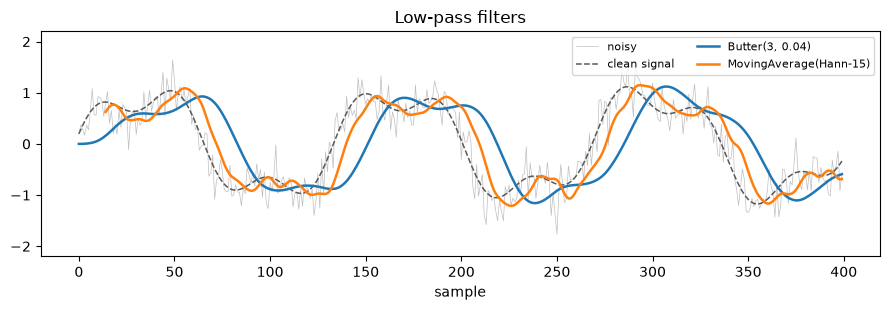
These are designed in the frequency domain: keep the slow variation, attenuate fast wiggles above a cutoff. Butter is a Butterworth IIR filter; a low order already gives a sharp roll-off and the filter carries only a few state values however long it runs. MovingAverage is an FIR filter you define by its tap weights, here a raised-cosine (Hann) window, giving a smooth, stable response with no feedback.

Low-pass filters give you direct control over which frequencies survive. Window-based statistics set the cutoff only implicitly through their width. The trade-off: a Butterworth's phase delay grows with its order and it can overshoot just after a sharp step, and an FIR needs many taps to make its cutoff steep. Both treat a spike as signal, so they are sensitive to outliers.

hann = np.hanning(15)
show("Low-pass filters", {
    "Butter(3, 0.04)":            Butter(3, 0.04)(noisy),
    "MovingAverage(Hann-15)":     MovingAverage((hann / hann.sum()).tolist())(noisy),
})

Local linear fit

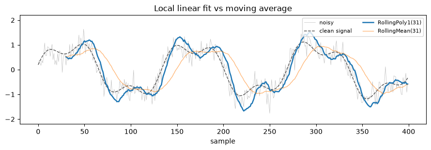
Instead of averaging the window, RollingPoly1 fits a straight line to it by least squares and returns the line's value at the most recent sample. Evaluating the fit at the leading edge rather than the middle removes most of the lag a moving average shows on a trending or ramping signal. Pass derivative_order=1 to get the slope directly from the same fit.

The cost: it lets a little more noise through than a plain mean, because it extrapolates to the edge rather than smoothing to the center.

show("Local linear fit vs moving average", {
    "RollingPoly1(31)":  RollingPoly1(W)(noisy),
    "RollingMean(31)":   RollingMean(W)(noisy),   # shown faint, for contrast
}, faint={"RollingMean(31)"})

Local quadratic fit

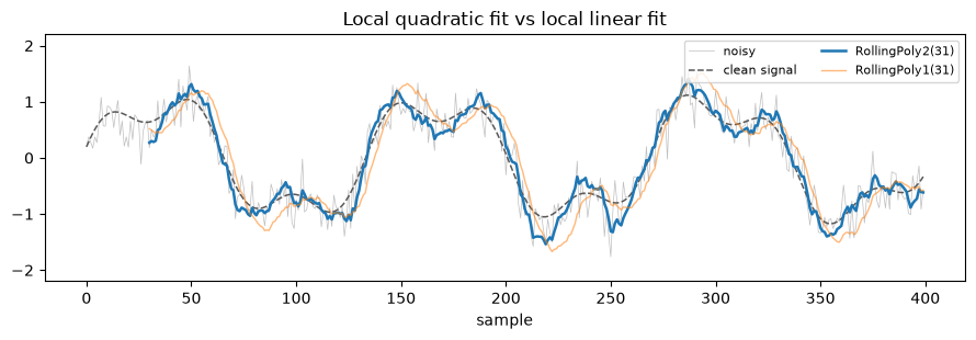
RollingPoly2 fits a parabola to the window, so it can follow curvature that a straight line cannot. Around peaks and troughs, where a moving average flattens the extreme and a linear fit cuts the corner, the quadratic holds the height and shape with very little lag. Pass derivative_order=2 to get the curvature directly; it is the causal counterpart of a Savitzky-Golay smoother.

More flexibility means more noise passes through, so on flat stretches a quadratic fit is less smooth than the mean or the linear fit. Use it when preserving the size and timing of features matters more than maximum smoothness.

show("Local quadratic fit vs local linear fit", {
    "RollingPoly2(31)":  RollingPoly2(W)(noisy),
    "RollingPoly1(31)":  RollingPoly1(W)(noisy),   # shown faint, for contrast
}, faint={"RollingPoly1(31)"})

Removing outliers before denoising

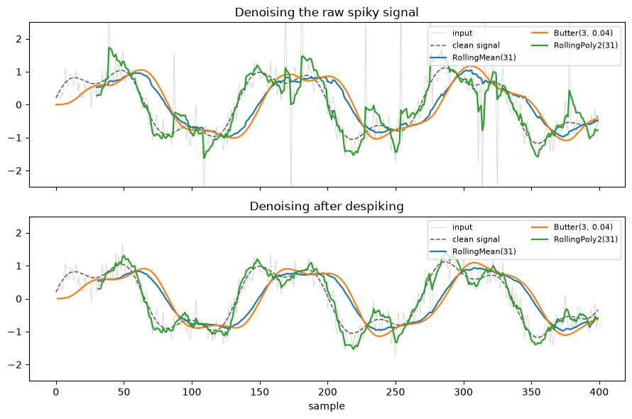
Real data often carries the occasional spike: a sensor glitch, a bad tick, a dropped packet. Every filter above except the median treats a spike as signal and lets it through, so a single outlier leaves a bump that lasts a full window.

Remove the spikes first and any of these smoothers can cope. The trick is to detect a spike by what defines it: a large and isolated jump. In the slowly varying level a spike is easy to miss, because the signal itself swings by a similar amount over a window. In the sample-to-sample change it stands out sharply: the smooth signal barely moves between neighbours while a spike leaps and springs back. screamer has this built in as ImpulseClip: it flags jumps far larger than the local noise (measured robustly on the first difference) and replaces those samples with the rolling median. The same three denoisers run on the raw spiky signal (top panel) and on the ImpulseClip-cleaned signal (bottom).

spiky = noisy.copy()
hit = rng.choice(n, 14, replace=False)
spiky[hit] += rng.choice([-1.0, 1.0], hit.size) * rng.uniform(2.5, 4.0, hit.size)

cleaned = ImpulseClip(window_size=31, n_sigma=4.0, start_policy="expanding")(spiky)

fig, (ax_raw, ax_clean) = plt.subplots(2, 1, figsize=(9, 6), sharex=True)
for ax, source, title in [(ax_raw,   spiky,   "Denoising the raw spiky signal"),
                          (ax_clean, cleaned, "Denoising after despiking")]:
    ax.plot(source, lw=0.5, color="0.8", label="input")
    ax.plot(clean, lw=1.1, color="0.35", ls="--", label="clean signal")
    for name, f in {"RollingMean(31)":  RollingMean(W),
                    "Butter(3, 0.04)":  Butter(3, 0.04),
                    "RollingPoly2(31)": RollingPoly2(W)}.items():
        ax.plot(f(source), lw=1.6, label=name)   # fresh functors per panel
    ax.set_title(title)
    ax.set_ylim(-2.5, 2.5)
    ax.legend(loc="upper right", fontsize=8, ncol=2)
ax_clean.set_xlabel("sample")
plt.tight_layout()

Choosing a filter

Family	Strong at	Watch out for
RollingMean, EwMean	smoothest result, cheapest to run	lag; one outlier smears across a window
RollingMedian	ignores spikes, keeps edges sharp	more compute; rougher than a mean on plain noise
Butter, MovingAverage	direct control of the frequency cutoff	phase delay and overshoot; not robust to outliers
RollingPoly1	little lag on trends; gives the slope	passes more noise than a mean
RollingPoly2	preserves peak height and timing; gives curvature	least smooth on flat stretches

For every filter and its parameters, see the Smoothing filters section of the reference.