Window statistics: rolling, exponential, expanding

screamer has three window families for moment-based statistics. A rolling window takes the last n samples with equal weight and a fixed lookback. Exponential weighting gives each sample a geometrically decaying weight, so recent values count more and no hard cutoff is needed. An expanding window grows from the first sample to the current one and never discards anything, making it the natural choice for session-to-date or all-time metrics; call .reset() to restart it between episodes.

The families make different trade-offs. Rolling has a clean, interpretable lookback and matches pandas numerically. Exponential reacts faster without committing to a hard cutoff. Expanding improves as data accumulates rather than dropping old samples. All three share the calling convention from notebook 1.

import numpy as np
import matplotlib.pyplot as plt
from screamer import RollingMean, RollingStd, EwMean, EwStd
from screamer import ExpandingMean, ExpandingStd, RollingCorr

rng = np.random.default_rng(0)
price = 100 + np.cumsum(rng.standard_normal(300))

Rolling and exponential weighting

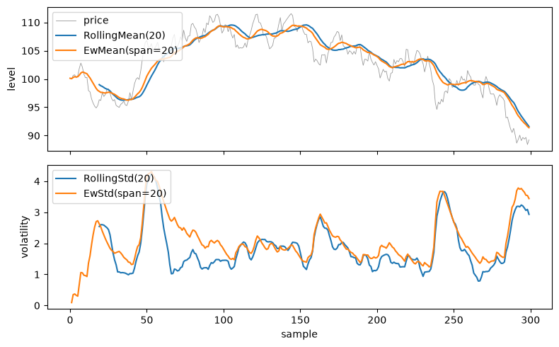
With a matched window and span of 20, the two families track the series differently. The exponential mean hugs recent moves while the rolling mean lags (top panel), and the exponential std reacts to a burst sooner and relaxes more smoothly (bottom). If an exact, interpretable lookback matters, use rolling; if faster response does, use exponential weighting.

roll_mean = RollingMean(20)(price)
ew_mean   = EwMean(span=20)(price)
roll_std  = RollingStd(20)(price)
ew_std    = EwStd(span=20)(price)

fig, (ax_level, ax_vol) = plt.subplots(2, 1, figsize=(8, 5), sharex=True)

ax_level.plot(price, lw=0.6, color="0.6", label="price")
ax_level.plot(roll_mean, label="RollingMean(20)")
ax_level.plot(ew_mean, label="EwMean(span=20)")
ax_level.set_ylabel("level")
ax_level.legend(loc="upper left")

ax_vol.plot(roll_std, label="RollingStd(20)")
ax_vol.plot(ew_std, label="EwStd(span=20)")
ax_vol.set_ylabel("volatility")
ax_vol.set_xlabel("sample")
ax_vol.legend(loc="upper left")

plt.tight_layout()

Warm-up behavior

A rolling window has nothing to report until it is full, so RollingMean(20) emits NaN for the first 19 samples. Exponential weighting has a value from the very first sample, though it takes roughly a span to settle. You can change the rolling window's warm-up with the start_policy argument; see NaN and warmup.

print("rolling first 3:", roll_mean[:3].round(3))   # NaN until the window fills
print("ew first 3     :", ew_mean[:3].round(3))     # a value from sample 0

rolling first 3: [nan nan nan]
ew first 3     : [100.126 100.056 100.268]

Same numbers as pandas

The rolling family is numerically identical to pandas, so results from pd.Series.rolling() carry over directly. Exponential-weighting conventions vary between libraries, so the EW family is not a drop-in for pandas ewm; see conventions for the details.

Expanding window: growing from the first sample

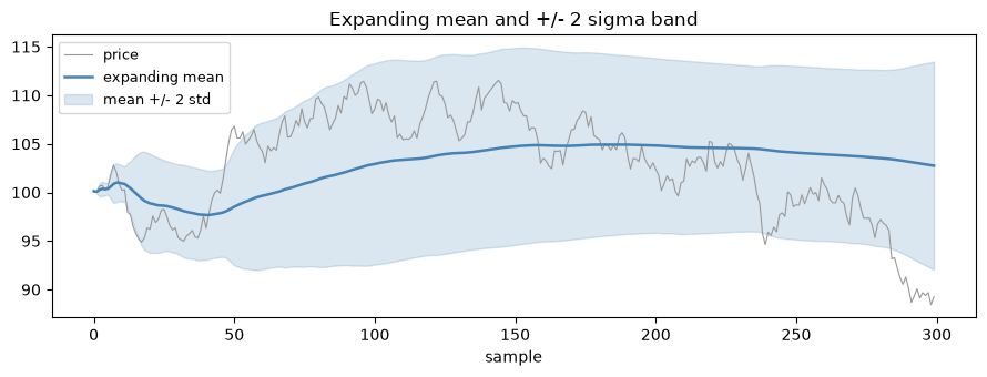
An expanding statistic includes everything from the first sample to the current one, so each new sample refines the estimate rather than replacing an old one. The mean settles quickly; the standard deviation band narrows as the estimate improves.

Use expanding statistics for session-to-date or all-time metrics: a running mean, a cumulative maximum, or a full-history standard deviation.

emean = ExpandingMean()(price)
estd  = ExpandingStd()(price)

fig, ax = plt.subplots(figsize=(9, 3.5))
ax.plot(price, lw=0.8, color="0.6", label="price")
ax.plot(emean, lw=1.8, color="steelblue", label="expanding mean")
ax.fill_between(
    np.arange(len(price)),
    emean - 2 * estd,
    emean + 2 * estd,
    alpha=0.20,
    color="steelblue",
    label="mean +/- 2 std",
)
ax.set_xlabel("sample")
ax.set_title("Expanding mean and +/- 2 sigma band")
ax.legend(fontsize=9)
plt.tight_layout()

Resetting between sessions with .reset()

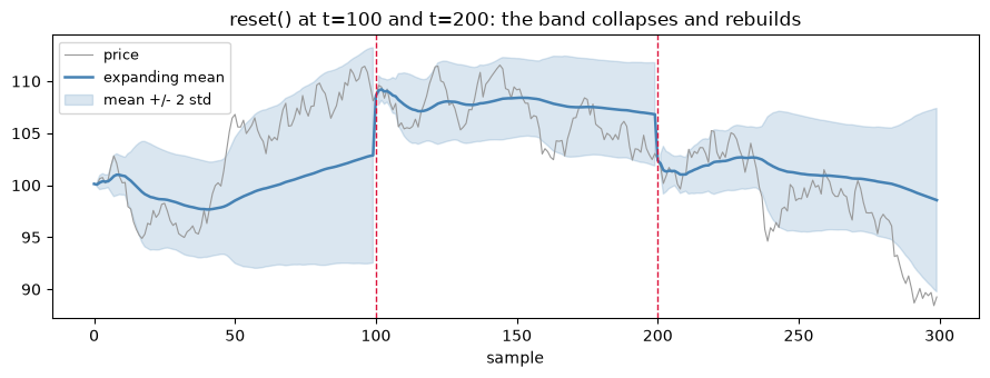
Expanding statistics accumulate over all history. Call .reset() to restart them, for example at the open of each trading session. Resetting the expanding mean and std at t = 100 and t = 200 starts each segment from scratch, so the band collapses at each reset and then rebuilds as new samples arrive.

# Reset at t=100 and t=200 by running each segment through the same accumulator.
# Each segment is an array call. .reset() clears state between segments so each starts fresh.
resets = [0, 100, 200, len(price)]
em, es = ExpandingMean(), ExpandingStd()
means, stds = [], []
for a, b in zip(resets[:-1], resets[1:]):
    means.append(np.asarray(em(price[a:b])))
    stds.append(np.asarray(es(price[a:b])))
    em.reset(); es.reset()
emean_r = np.concatenate(means)
estd_r  = np.concatenate(stds)

fig, ax = plt.subplots(figsize=(9, 3.5))
ax.plot(price, lw=0.8, color="0.6", label="price")
ax.plot(emean_r, lw=1.8, color="steelblue", label="expanding mean")
ax.fill_between(
    np.arange(len(price)),
    emean_r - 2 * estd_r,
    emean_r + 2 * estd_r,
    alpha=0.20, color="steelblue", label="mean +/- 2 std",
)
for r in (100, 200):
    ax.axvline(r, color="crimson", lw=1.0, ls="--")
ax.set_xlabel("sample")
ax.set_title("reset() at t=100 and t=200: the band collapses and rebuilds")
ax.legend(fontsize=9)
plt.tight_layout()

Two-input operators: rolling correlation

Some operators take two input streams and produce one. RollingCorr(window) computes the Pearson correlation between two co-indexed series over a rolling window, so you pass both series as separate arguments.

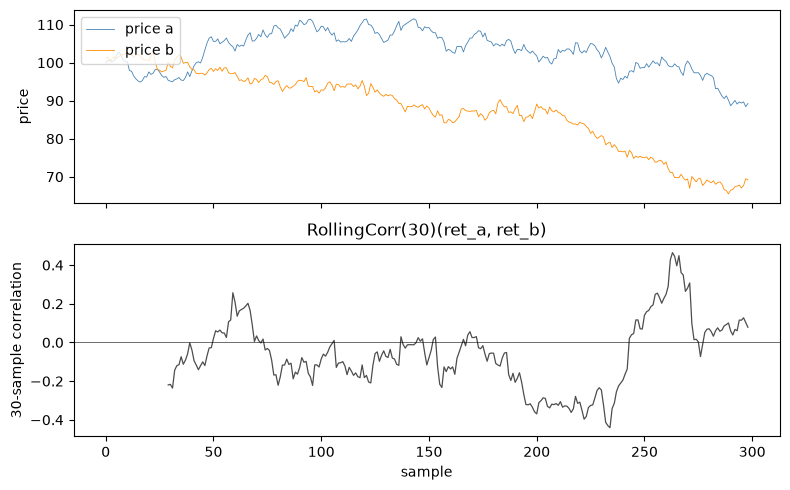
Below, two independent price streams show no stable correlation; the rolling window makes that variation visible.

rng2 = np.random.default_rng(1)
price_b = 100 + np.cumsum(rng2.standard_normal(len(price)))
ret_a = np.diff(price)        # returns of series a
ret_b = np.diff(price_b)      # returns of series b (independent)
rolling_corr = RollingCorr(30)(ret_a, ret_b)

fig, (ax_p, ax_c) = plt.subplots(2, 1, figsize=(8, 5), sharex=True)
ax_p.plot(price[1:], lw=0.6, color="steelblue", label="price a")
ax_p.plot(price_b[1:], lw=0.6, color="darkorange", label="price b")
ax_p.set_ylabel("price")
ax_p.legend(loc="upper left")

ax_c.plot(rolling_corr, lw=0.9, color="0.3")
ax_c.axhline(0, color="k", lw=0.4)
ax_c.set_ylabel("30-sample correlation")
ax_c.set_xlabel("sample")
ax_c.set_title("RollingCorr(30)(ret_a, ret_b)")

plt.tight_layout()
print("first non-NaN at sample", np.argmax(~np.isnan(rolling_corr)))

first non-NaN at sample 29

The window-statistics family

The three families cover the main moment-based statistics. Where a cell is empty, that statistic has no natural form in that window style.

statistic	Rolling	Exponentially-weighted	Expanding
mean	RollingMean	EwMean	ExpandingMean
std / var	RollingStd, RollingVar	EwStd, EwVar	ExpandingStd, ExpandingVar
z-score	RollingZscore	EwZscore
skew / kurtosis	RollingSkew, RollingKurt	EwSkew, EwKurt	ExpandingSkew, ExpandingKurt
rms	RollingRms	EwRms
sum	RollingSum		ExpandingSum
min / max	RollingMin, RollingMax		ExpandingMin, ExpandingMax
median / quantile	RollingMedian, RollingQuantile
correlation	RollingCorr

For the complete list including financial indicators and OHLC volatility estimators, see the function reference.